Thread
分布式训练
S - 单个 GPU 训练
T - 只需要将张量传输到同一个 GPU 设备上,PyTorch 会处理其余的工作
将Tensor和Model传输到同一个 GPU 设备上, PyTorch 会处理其余的工作
- 计算在GPU
- 输出的 logits 也自然会在 GPU 上。
回到CPU
- 如果你要将 GPU 张量传给 NumPy、Pandas、Matplotlib 等非 PyTorch 库,就必须显式 .cpu(),否则会报错。
- 自动拷贝只发生在 print() 或 str() 等只读操作中。
- 可以直接 print() GPU 上的张量,不需要先手动把它 .cpu() 回主机内存。PyTorch 会自动在后台把数据从 GPU 拷贝到 CPU,以便打印。
A
Basic
tensor_1 = torch.tensor([1., 2., 3.])
tensor_2 = torch.tensor([4., 5., 6.])
print(tensor_1 + tensor_2)  # 有两个张量可以相加。默认情况下,这个计算将在 CPU 上执行:
# tensor([5., 7., 9.])


# 如果一个 PyTorch 张量存放在某个设备上,那么其操作也会在同一个设备上执行
# 将这些张量转移到 GPU 上  .to("cuda")、.to("cuda:0")、.to("cuda:1")
tensor_1 = tensor_1.to("cuda")
tensor_2 = tensor_2.to("cuda")
print(tensor_1 + tensor_2)  # 在GPU执行加法操作
# tensor([5., 7., 9.], device='cuda:0')


# 所有的张量必须位于同一个设备上。否则,如果一个张量位于 CPU,另一个张量位于 GPU,计算就会失败
tensor_1 = tensor_1.to("cpu")
print(tensor_1 + tensor_2)
tensor and model
import torch.nn.functional as F


torch.manual_seed(123)
model = NeuralNetwork(num_inputs=2, num_outputs=2)

device = torch.device("cuda" if torch.cuda.is_available() else "cpu") # NEW
model.to(device) # NEW

optimizer = torch.optim.SGD(model.parameters(), lr=0.5)

num_epochs = 3

for epoch in range(num_epochs):

    model.train()
    for batch_idx, (features, labels) in enumerate(train_loader):

        features, labels = features.to(device), labels.to(device) # NEW
        # 在当前修改后的训练循环中,由于从 CPU 转移到 GPU的内存传输成本,我们可能不会看到速度的提升。然而,我们可以期待在训练深度神经网络,尤其是大语言模型时,会有显著的速度提升。
        logits = model(features)
        loss = F.cross_entropy(logits, labels) # Loss function

        optimizer.zero_grad()
        loss.backward()
        optimizer.step()

        ### LOGGING
        print(f"Epoch: {epoch+1:03d}/{num_epochs:03d}"
              f" | Batch {batch_idx:03d}/{len(train_loader):03d}"
              f" | Train/Val Loss: {loss:.2f}")

    model.eval()
S - 多个 GPU 训练
- 分布式训练的概念是将模型训练分配到多个机器的多个 GPU上
T - PyTorch的分布式数据并行(DistributedDataParallel,DDP)策略
分数据,共享梯度

- 模型复制传输到GPUs - PyTorch 会在每个 GPU 上启动一个独立的进程,每个进程都会接收并保存一份模型副本
- 数据分割传输到GPUs - 每个模型都会从数据加载器中接收一个小批次(或简称“批次”) 数据。可以使用 DistributedSampler 来确保在使用 DDP 时,每个 GPU 接收到的批次不同且不重叠

- 由于每个模型副本会看到不同的训练数据样本,因此前向传播和反向传播在每个 GPU 上独立执行。
- 一旦前向传播和反向传播完成,每个 GPU 上各个模型副本的梯度会在所有GPU 之间同步。这可以确保每个模型副本具有相同的更新权重,可以确保模型不会出现分歧
rank
- 这个词来源于 MPI(Message Passing Interface),这是一个早期的并行计算标准。在 MPI 中:
- 每个进程在通信组(communicator)中都有一个编号。
- 这个编号就叫做 rank,意思是“在这个组中的位置”,从 0 到 world_size - 1
- 如果你有 2 张 GPU,那么:
- rank=0 表示第一个进程(通常绑定 GPU 0)
- rank=1 表示第二个进程(通常绑定 GPU 1)
一GPU一进程(官方推荐的做法,也是业界主流的分布式训练方式)
- DDP 的设计初衷就是每个 GPU 对应一个进程
- 能最大化 GPU 利用率和通信效率
一GPU多进程(不常见)
- 可能导致资源竞争、上下文切换开销大
A
1.限制能用的GPU
- 在多 GPU 机器上限制用于训练的 GPU 数量,那么最简单的方法是使用CUDA_VISIBLE_DEVICES 环境变量
# 如果你的机器有 4 个 GPU,而你只想使用第一个和第三个 GPU
CUDA_VISIBLE_DEVICES=0,2 python xxx.py
2.按照GPU数量,启动多个进程
- 使用 torch.cuda.device_count() 打印可用 GPU的数量作为world_size
- 使用 PyTorch的 multiprocessing.spawn 函数生成新进程
- nproces=world_size - 为每个 GPU 启动一个进程
- main - 用这些进程启动主函数main,并通过args 提供一些额外的参数。
- main 的第一个参数 rank 是由 mp.spawn 自动传入的,表示当前进程的编号(从 0 到 world_size - 1)。main 实际上是这样被调用的:
- main(rank=0,world_size,num_epochs)
- main(rank=1,world_size,num_epochs)
- …
- main(rank=world_size-1,world_size,num_epochs)
if __name__ == "__main__":
    torch.manual_seed(123)
    num_epochs = 3
    world_size = torch.cuda.device_count()
    mp.spawn(main, args=(world_size, num_epochs), nprocs=world_size)
3.将每个进程加入到进程组并绑定到各自GPU
- 设置主节点的地址和端口以便不同进程之间进行通信
- 在单机多卡训练中,localhost 表示本机。
- 所有进程会通过这个地址和端口建立通信连接。
- init_process_group- 加入同一个进程组,并完成自身的初始化。
- init_method - 初始化方法env://, topc://ip.port
- backend - 通信后端nccl, mpi, gloo
- rank - 当前进程编号,0~world_size -1
- world_size - 总进程数
- 将当前进程绑定到编号为 rank 的 GPU
- 如果你有 4 张 GPU,rank 为 0 的进程就用 cuda:0,rank 为 1 的进程就用 cuda:1,以此类推
def ddp_setup(rank, world_size):
    os.environ["MASTER_ADDR"] = "localhost"
    os.environ["MASTER_PORT"] = "12345"

    init_process_group(backend="nccl", rank=rank, world_size=world_size)

    torch.cuda.set_device(rank)
4.每个进程接受子样本
- 在训练加载器中设置 sampler=DistributedSampler(train_ds) 每个 GPU 将接收不同的训练数据子样本
def prepare_dataset():
    X_train = torch.tensor([
        [-1.2, 3.1],
        [-0.9, 2.9],
        [-0.5, 2.6],
        [2.3, -1.1],
        [2.7, -1.5]
    ])
    y_train = torch.tensor([0, 0, 0, 1, 1])

    X_test = torch.tensor([
        [-0.8, 2.8],
        [2.6, -1.6],
    ])
    y_test = torch.tensor([0, 1])


    train_ds = ToyDataset(X_train, y_train)
    test_ds = ToyDataset(X_test, y_test)

    train_loader = DataLoader(
        dataset=train_ds,
        batch_size=2,
        shuffle=False,  # NEW: False because of DistributedSampler below
        pin_memory=True,
        drop_last=True,
        sampler=DistributedSampler(train_ds)  # NEW
    )
    test_loader = DataLoader(
        dataset=test_ds,
        batch_size=2,
        shuffle=False,
    )
    return train_loader, test_loader
5.每个进程单独训练
- 通过.to(rank) 将模型和数据传输到目标设备,其中 rank 用于指代 GPU 设备 ID
- 通过DDP 封装模型,从而在训练期间实现不同 GPU 之间梯度的同步
- train_loader Set sampler to ensure each epoch has a different shuffle order
- 评估模型后,使用 destroy_process_group() 来干净地退出分布式训练模式并释放已分配的资源
def main(rank, world_size, num_epochs):

    ddp_setup(rank, world_size)  # NEW: initialize process groups

    train_loader, test_loader = prepare_dataset()
    model = NeuralNetwork(num_inputs=2, num_outputs=2)
    model.to(rank)
    optimizer = torch.optim.SGD(model.parameters(), lr=0.5)

    model = DDP(model, device_ids=[rank])  # NEW

    for epoch in range(num_epochs):
        train_loader.sampler.set_epoch(epoch) # NEW

        model.train()
        for features, labels in train_loader:

            features, labels = features.to(rank), labels.to(rank)  # New
            logits = model(features)
            loss = F.cross_entropy(logits, labels)  # Loss function

            optimizer.zero_grad()
            loss.backward()
            optimizer.step()

            # LOGGING
            print(f"[GPU{rank}] Epoch: {epoch+1:03d}/{num_epochs:03d}"
                  f" | Batchsize {labels.shape[0]:03d}"
                  f" | Train/Val Loss: {loss:.2f}")

    model.eval()

    try:
        train_acc = compute_accuracy(model, train_loader, device=rank)
        print(f"[GPU{rank}] Training accuracy", train_acc)
        test_acc = compute_accuracy(model, test_loader, device=rank)
        print(f"[GPU{rank}] Test accuracy", test_acc)

    destroy_process_group()  # NEW
6.summary
import torch
import torch.nn.functional as F
from torch.utils.data import Dataset, DataLoader

# NEW imports:
import os
import platform
import torch.multiprocessing as mp
from torch.utils.data.distributed import DistributedSampler
from torch.nn.parallel import DistributedDataParallel as DDP
from torch.distributed import init_process_group, destroy_process_group


# NEW: function to initialize a distributed process group (1 process / GPU)
# this allows communication among processes
def ddp_setup(rank, world_size):
    """
    Arguments:
        rank: a unique process ID
        world_size: total number of processes in the group
    """
    # rank of machine running rank:0 process
    # here, we assume all GPUs are on the same machine
    os.environ["MASTER_ADDR"] = "localhost"
    # any free port on the machine
    os.environ["MASTER_PORT"] = "12345"

    # initialize process group
    if platform.system() == "Windows":
        # Disable libuv because PyTorch for Windows isn't built with support
        os.environ["USE_LIBUV"] = "0"
        # Windows users may have to use "gloo" instead of "nccl" as backend
        # gloo: Facebook Collective Communication Library
        init_process_group(backend="gloo", rank=rank, world_size=world_size)
    else:
        # nccl: NVIDIA Collective Communication Library
        init_process_group(backend="nccl", rank=rank, world_size=world_size)

    torch.cuda.set_device(rank)


class ToyDataset(Dataset):
    def __init__(self, X, y):
        self.features = X
        self.labels = y

    def __getitem__(self, index):
        one_x = self.features[index]
        one_y = self.labels[index]
        return one_x, one_y

    def __len__(self):
        return self.labels.shape[0]


class NeuralNetwork(torch.nn.Module):
    def __init__(self, num_inputs, num_outputs):
        super().__init__()

        self.layers = torch.nn.Sequential(
            # 1st hidden layer
            torch.nn.Linear(num_inputs, 30),
            torch.nn.ReLU(),

            # 2nd hidden layer
            torch.nn.Linear(30, 20),
            torch.nn.ReLU(),

            # output layer
            torch.nn.Linear(20, num_outputs),
        )

    def forward(self, x):
        logits = self.layers(x)
        return logits


def prepare_dataset():
    X_train = torch.tensor([
        [-1.2, 3.1],
        [-0.9, 2.9],
        [-0.5, 2.6],
        [2.3, -1.1],
        [2.7, -1.5]
    ])
    y_train = torch.tensor([0, 0, 0, 1, 1])

    X_test = torch.tensor([
        [-0.8, 2.8],
        [2.6, -1.6],
    ])
    y_test = torch.tensor([0, 1])

    # Uncomment these lines to increase the dataset size to run this script on up to 8 GPUs:
    # factor = 4
    # X_train = torch.cat([X_train + torch.randn_like(X_train) * 0.1 for _ in range(factor)])
    # y_train = y_train.repeat(factor)
    # X_test = torch.cat([X_test + torch.randn_like(X_test) * 0.1 for _ in range(factor)])
    # y_test = y_test.repeat(factor)

    train_ds = ToyDataset(X_train, y_train)
    test_ds = ToyDataset(X_test, y_test)

    train_loader = DataLoader(
        dataset=train_ds,
        batch_size=2,
        shuffle=False,  # NEW: False because of DistributedSampler below
        pin_memory=True,
        drop_last=True,
        # NEW: chunk batches across GPUs without overlapping samples:
        sampler=DistributedSampler(train_ds)  # NEW
    )
    test_loader = DataLoader(
        dataset=test_ds,
        batch_size=2,
        shuffle=False,
    )
    return train_loader, test_loader


# NEW: wrapper
def main(rank, world_size, num_epochs):

    ddp_setup(rank, world_size)  # NEW: initialize process groups

    train_loader, test_loader = prepare_dataset()
    model = NeuralNetwork(num_inputs=2, num_outputs=2)
    model.to(rank)
    optimizer = torch.optim.SGD(model.parameters(), lr=0.5)

    model = DDP(model, device_ids=[rank])  # NEW: wrap model with DDP
    # the core model is now accessible as model.module

    for epoch in range(num_epochs):
        # NEW: Set sampler to ensure each epoch has a different shuffle order
        train_loader.sampler.set_epoch(epoch)

        model.train()
        for features, labels in train_loader:

            features, labels = features.to(rank), labels.to(rank)  # New: use rank
            logits = model(features)
            loss = F.cross_entropy(logits, labels)  # Loss function

            optimizer.zero_grad()
            loss.backward()
            optimizer.step()

            # LOGGING
            print(f"[GPU{rank}] Epoch: {epoch+1:03d}/{num_epochs:03d}"
                  f" | Batchsize {labels.shape[0]:03d}"
                  f" | Train/Val Loss: {loss:.2f}")

    model.eval()

    try:
        train_acc = compute_accuracy(model, train_loader, device=rank)
        print(f"[GPU{rank}] Training accuracy", train_acc)
        test_acc = compute_accuracy(model, test_loader, device=rank)
        print(f"[GPU{rank}] Test accuracy", test_acc)

    ####################################################
    # NEW (not in the book):
    except ZeroDivisionError as e:
        raise ZeroDivisionError(
            f"{e}\n\nThis script is designed for 2 GPUs. You can run it as:\n"
            "CUDA_VISIBLE_DEVICES=0,1 python DDP-script.py\n"
            f"Or, to run it on {torch.cuda.device_count()} GPUs, uncomment the code on lines 103 to 107."
        )
    ####################################################

    destroy_process_group()  # NEW: cleanly exit distributed mode


def compute_accuracy(model, dataloader, device):
    model = model.eval()
    correct = 0.0
    total_examples = 0

    for idx, (features, labels) in enumerate(dataloader):
        features, labels = features.to(device), labels.to(device)

        with torch.no_grad():
            logits = model(features)
        predictions = torch.argmax(logits, dim=1)
        compare = labels == predictions
        correct += torch.sum(compare)
        total_examples += len(compare)
    return (correct / total_examples).item()


if __name__ == "__main__":
    # This script may not work for GPUs > 2 due to the small dataset
    # Run `CUDA_VISIBLE_DEVICES=0,1 python DDP-script.py` if you have GPUs > 2
    print("PyTorch version:", torch.__version__)
    print("CUDA available:", torch.cuda.is_available())
    print("Number of GPUs available:", torch.cuda.device_count())
    torch.manual_seed(123)

    # NEW: spawn new processes
    # note that spawn will automatically pass the rank
    num_epochs = 3
    world_size = torch.cuda.device_count()
    mp.spawn(main, args=(world_size, num_epochs), nprocs=world_size)
    # nprocs=world_size spawns one process per GPU
R
除去设备之间由于使用 DDP 而产生的少量通信开销,理论上使用两个 GPU 可以将训练一轮的时间缩短一半。时间效率会随着 GPU 数量的增加而提高,如果有 8 个 GPU,那么可以将一轮的处理速度提高 8 倍,以此类推。
容量,增加core
数量, Increase in-flight instructions
S - How to saturate bandwidth
T - Little’s Law
For Escalator: Add more in-flight people to saturate bandwidth
- Bandwidth = 0.5 person/s
- Latency = 40 senconds
- One person in flight
- How many persons do we need in-flight to saturate bandwidth?
- Concurrency = Bandwidth * Latency = 0.5 * 40 = 20 persons

- Concurrency = Bandwidth * Latency = 0.5 * 40 = 20 persons
For GPU: Increase in-flight instructions to maximize performance
- FP32 Bandwidth = 8 ops per cycle
- FP32 Latency = 24 cycles
- Concurrency = 8 * 24 operations in-flight
- Increase in-flight instructions -> hide latency of compute & memory access -> saturate compute units & memory bandwidth -> maximize performance
Ways to increase in-flight instructions
- More threads by improving TLP
- More independent instructions per thread by improving ILP
S - Improving ILP by computing more elements per thread to merge instruction issue
- 用#prama unroll, 展开且合并两组独立的load指令
- 用常量使idx可静态分析,合并要写元素的load
Instruction Issue指令发射
1.一句话通常是一条指令 2.常见指令
| 指令 | 功能描述 | 示例语句 | 说明 |
|---|---|---|---|
LDG(Load Global) |
从全局内存加载数据到寄存器 | ld.global.f32 %f1, [%r1]; |
将 %r1 指向的内存地址中的 float 加载到 %f1 |
STG(Store Global) |
将寄存器中的数据写入全局内存 | st.global.f32 [%r1], %f2; |
把 %f2 中的 float 写入 %r1 指定的全局内存地址 |
FFMA(Fused Floating-point Multiply-Add融合乘加) |
执行 a * b + c 操作 |
ffma.f32 %f3, %f1, %f2, %f4; |
%f3 = %f1 * %f2 + %f4,提高精度和性能 |
3.Instruction Issue(指令发射)是指将指令从指令队列发送到执行单元(如 ALU、SFU、Load/Store 单元等)的过程
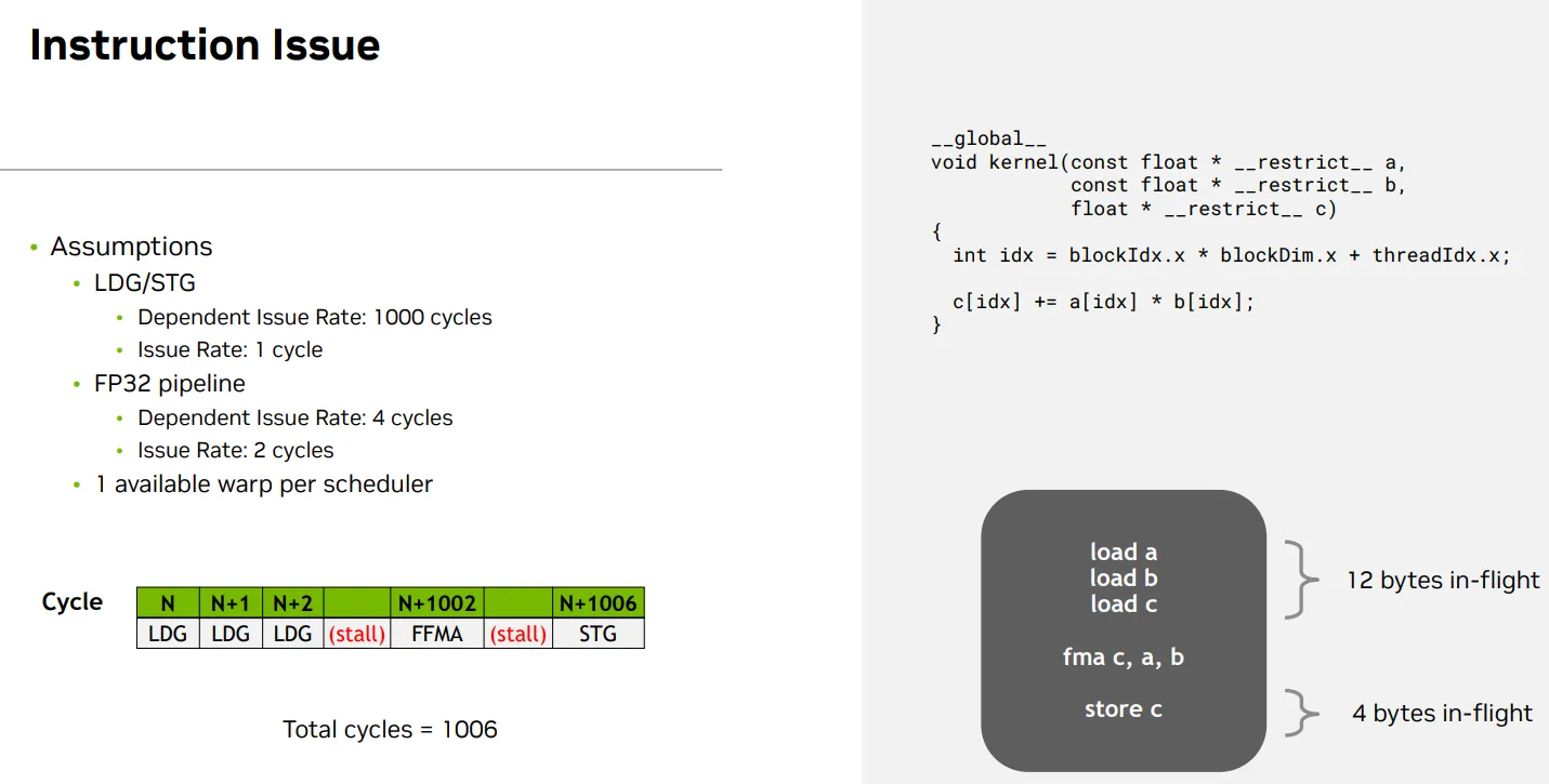
假设
- LDG/STG(全局内存加载/存储)
- Issue Rate: 每 1 cycle 可发射一次
- Dependent Issue Rate: 1000 cycles(即依赖数据的下一条指令必须等 1000 cycles 才能发射)
- FP32 Pipeline(浮点计算)
- Issue Rate: 每 2 cycles 可发射一次
- Dependent Issue Rate: 4 cycles(即依赖前一条 FP32 指令的下一条指令需等 4 cycles)
- 每个调度器只有一个 warp 可用
发射
- Cycle N ~ N+2:连续发射了 3 条 LDG 指令(加载 a[idx], b[idx], c[idx])
- 由于 LDG 的 issue rate 是 1 cycle,所以可以连续发射。
- 但这些加载的数据是后续 FFMA 所依赖的,因此必须等待 1000 cycles 才能发射 FFMA。
- Cycle N+3~1001:出现了 (stall),表示由于数据依赖,调度器无法发射新的指令。
- Cycle N+1002:执行 FFMA(浮点乘加)
- 由于 LDG 的 dependent latency 是 1000 cycles,FFMA 必须等到 N+1002 才能执行。
- 如果下一条指令依赖 FFMA 的结果(无论它是不是 FP32 运算),它必须等 4 个 cycles 才能发射。
- Cycle N+1006:执行 STG(将结果写回全局内存)
- STG 依赖 FFMA 的结果,因此必须等 FFMA 完成后再等 4 cycles(FP32 dependent latency)才能发射。
- STG 本身是 memory 操作,符合其 issue 和 dependent 规则。
总结
- 总共是1006个cycle
- 由于 全局内存访问的高延迟(1000 cycles),导致即使指令可以快速发射,仍然需要等待数据准备好,最终一个线程处理两个元素的整个 pipeline 需要 1006 个周期
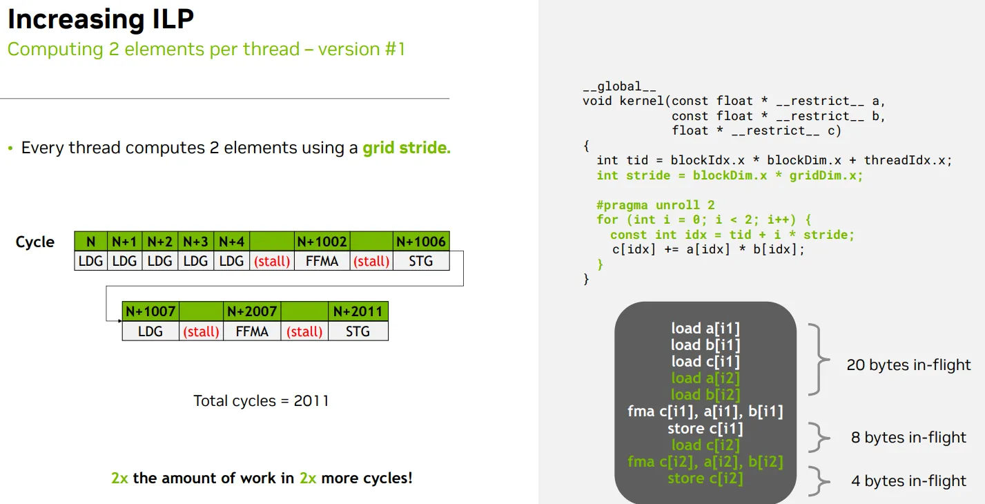
computing more elements per thread - 每个线程处理两个相隔 整个grid的线程总数/grid stride 的元素
- 不是说要用grid,本来就要用
- 是说要unroll 2, 展开并合并两组独立的指令,减少整体数据
- grid stride没问题只要数组长度 N 足够:例如至少为 2 * stride
BEFORE
- 每个线程只处理一个元素 idx
- a[idx] 和 b[idx] 的加载是 依赖于 idx 的计算
- c[idx] += … 是一个 读-改-写 操作,依赖于前面两个加载的结果
- 所以这三个操作之间是严格串行依赖的
int idx = blockIdx.x * blockDim.x + threadIdx.x;
c[idx] += a[idx] * b[idx];
AFTER
- 每个线程处理两个元素:idx1 = tid 和 idx2 = tid + stride
- 这两个元素之间没有数据依赖,可以并行调度
- 编译器看到 #pragma unroll 2,会将循环展开为两个独立的语句;
- a[idx] 和 b[idx],因为它们是 const float*,只读且 __ restrict __ 限定了它们不会别名冲突。
- 因此,load a[idx2] 和 load b[idx2] 可以在 load a[idx1] 和 load b[idx1] 之后立即发射,而不需要等待 FFMA 或 STG 完成。
int tid = blockIdx.x * blockDim.x + threadIdx.x;
int stride = blockDim.x * gridDim.x;
#pragma unroll 2
for (int i = 0; i < 2; i++) {
    const int idx = tid + i * stride;
    c[idx] += a[idx] * b[idx];
}
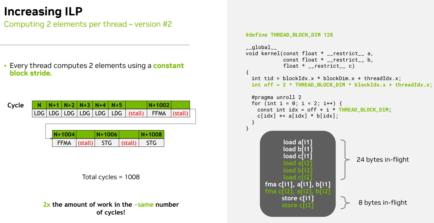
computing more elements per thread - 每个线程处理两个相隔 THREAD_BLOCK_DIM/constant block stride 的元素
地址计算是否静态可分析
- 可静态分析”并不是指编译器能知道它的具体值,而是指它的结构和取值范围是可预测的,从而允许编译器进行某些优化
- 为什么 blockIdx.x 是“可分析”的?
- 虽然 blockIdx.x 是运行时变量,但它的取值范围是 [0, gridDim.x - 1],而 gridDim.x 是在 host 端 kernel 启动时指定的,编译器知道它是一个固定的配置参数,不会在 kernel 内部改变。
- 这意味着:
- 编译器可以假设 blockIdx.x 是一个有限范围内的整数
- 可以在某些场景下进行循环展开或索引优化
- 为什么 gridDim.x 本身不可静态分析?
- gridDim.x 是由 host 端传入的配置参数
- 编译器无法在编译阶段知道它的具体值
BEFORE
- use dim
- 编译器无法在编译期判断 idx0 和 idx1 是否访问不同地址
- c[idx] += … 是一个 读-改-写(load-modify-store)操作
- 调度器可能采取更保守的策略,等待 FFMA(idx1) 和 store c[idx1] 完成后,才发射 load c[idx2],以避免潜在的地址冲突(即使实际上没有
int tid = blockIdx.x * blockDim.x + threadIdx.x;
int stride = blockDim.x * gridDim.x;
idx = tid + i * stride;
- use constant
- THREAD_BLOCK_DIM 是一个 编译期常量(通常是 #define 或 const int)
- i 是循环变量,循环次数固定(比如 for (int i = 0; i < 2; ++i))
- blockIdx.x 和 threadIdx.x 是 CUDA 内建变量,虽然它们是运行时值,但它们的 取值范围是已知的(比如 blockIdx.x ∈ [0, gridDim.x))
- 所以 off + i * THREAD_BLOCK_DIM 是一个线性表达式,不同线程的 off 值是互不重叠、线性分布的
- 编译器可以展开为多个具体的 idx 值
int off = 2 * THREAD_BLOCK_DIM * blockIdx.x + threadIdx.x;
const int idx = off + i * THREAD_BLOCK_DIM;
S - Improving TLP by increasing active warps num(occupancy) by relieving limiter
- 减少每个线程需要的存储,能创建更多的warp驻留在SM上,有更多的线程
| 资源类型 | 数值要求 | 说明 |
|---|---|---|
| 每线程寄存器数 | ≤ 32 | SM 总寄存器数通常为 65536;64 warp × 32线程 × 32寄存器 = 65536 |
| 每 block 共享内存使用 | ≤ 1.5 KB(推荐) | SM 的共享内存上限为 96KB(Ampere),如加载 64 warp(假设 256线程/block → 8warp/block)需加载 8 block,共享内存不得超过 96KB / 8 = 12KB/block,推荐进一步保守控制在 1.5KB/block 以内以预留空间 |
| block size(线程数) | 256 ~ 512(需为 32 的倍数) «<gridDim = 8, blockDim = 256»> | 保证 warp 整齐划分(32整数倍),并使 SM 能加载多个 block 以填满 warp 数。如 256线程/block → 8warp/block,需要 8 block 才能达到 64 warp |
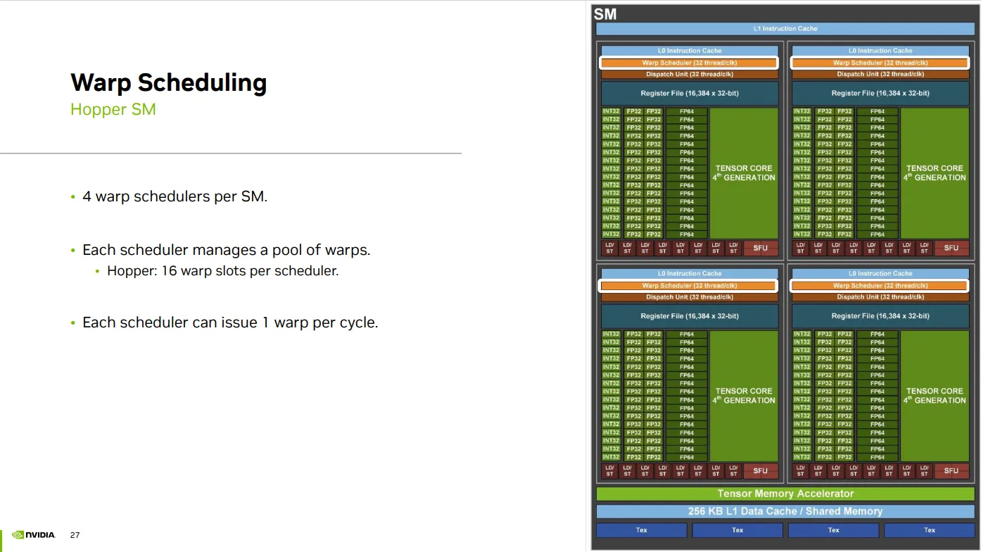
Warp scheduling for active warps num(occupancy)
Warp num
- 固定硬件上限, 每个 SM 理论上最多能容纳的 warp 数(如 64 warp) -> 最大 warp
- CUDA kernel 启动时,确实可以创建大量 warp(比如几千个) -> 可创建 warp 是理论数量
- 但每个 SM 的资源有限(寄存器、共享内存、线程数),所以只有部分 warp 能真正“驻留”在 SM 上,成为 活跃 warp -> 活跃 warp
Occupancy
- 每周期 issue 的 warp 数是调度器能力
- Occupancy 是指有多少 warp 被加载并准备运行(active)\
- 因为当有些 warp 因为访存而 stall,调度器可以切换到其他 warp:
- 有更多 warp ➜ 更容易隐藏内存延迟
- 少 warp ➜ 被访存 stall 卡住,就没别的 warp 可以执行 ➜ idle
- 因为当有些 warp 因为访存而 stall,调度器可以切换到其他 warp:
Each Warp scheduler
- has 16 warp slots, can manage 16 ready waprs
- issue 1 warp per cycle
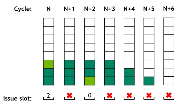
Active Warp states
- Stalled
- Eligible
- Selected/issue/active - Warps occupying scheduler warp slots
From eligible to active
- Each cycle: out of all eligible warps, select one to issue on that cycle.
- Warp at slot 2 becomes eligible. Warp at slot 2 is selected.
- Warp selected at cycle N is not eligible in cycle N+1
- E.g., instructions with longer latencies.
- No eligible warps! Issue slot unused
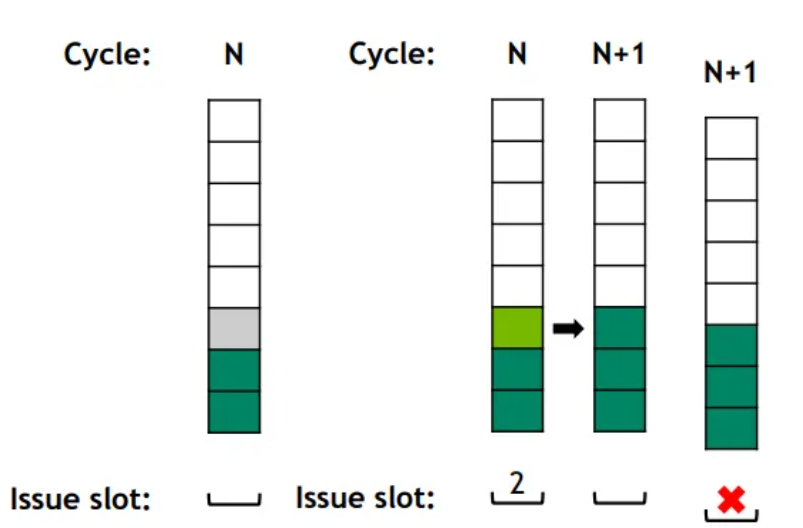
Having more active warps would help reduce idle issue slots and hide latencies of stalled warps.
Occupancy(占用率)- 一个 SM(Streaming Multiprocessor)上实际活跃的 warps 数量与其最大可支持 warps 数量的比值

Occupancy limiters
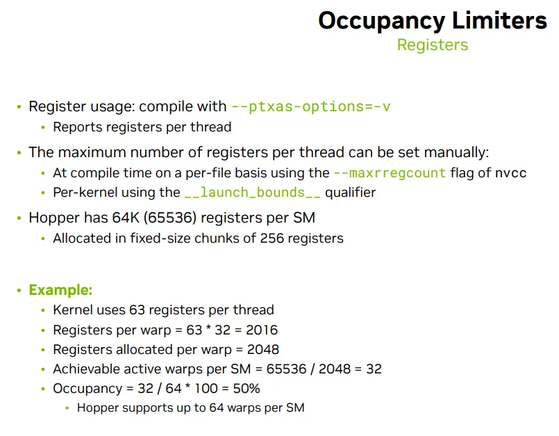
Register (Per SM, 64k 32bit registers)
- Each thread uses registers -> Registers per thread: 63, Registers per warp = 63 × 32 = 2016
- Registers are allocated in chunks (e.g., 256) -> Registers allocated per warp (rounded up to next multiple of 256): 2048
- total number of registers per SM is fixed (e.g., 65536) -> Total registers per SM: 65536
- The more registers each warp uses, the fewer warps can fit on an SM,Max active warps per SM = 65536 / 2048 = 32 warps
- Max possible warps per SM (on Hopper architecture): 64 warps
- Occupancy = 32 / 64 × 100% = 50%
- High register usage per thread reduces the number of warps that can be active on an SM, thereby lowering occupancy.
- 每线程使用 ≤ 32 个寄存器 是达到 64 warp occupancy 的关键条件之一。
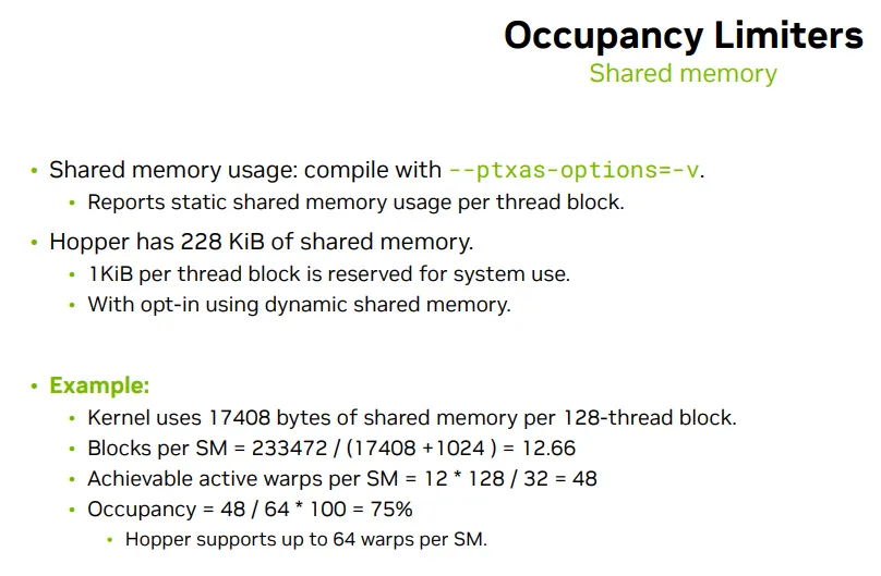
Shared memory (Per SM, 228KB)
- 每个 Block 的共享内存需求是每个kernel不一样的 - 比如,一个 128 线程的 block 使用 17408 字节 的共享内存,再加上 1024 字节 的额外开销,故每个 block 总共使用:17408 + 1024 = 18432 字节
- 每个 SM 总共提供 233472 字节 的共享内存 -> 每个 SM 能容纳的active Block数 Blocks per SM = 233472 / 18432} =12.66 由于实际运行中 block 数必须为整数,所以取整为 12 个 block。
- 每个SM active warp 数为:12 * 4 = 48 个 warp
- 在一个 SM 上有 12 个 block
- 每个 block 中有 128 个线程,而一个 warp 有 32 个线程,所以一个 block 内有: 128 / 32 = 4 个 warp
- Occupancy: 48/64=75%
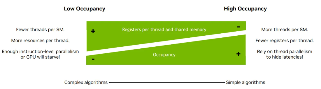
Tradeoff between TLP and ILP
Simple alogrithms, High TLP, High occupancy, Choose Fisrt
- more threads per SM
- fewer register per thread, fewer shared memory
Complex algorithms, High ILP
- fewere thread per SM
- more resources per thread
质量,Tensor Cores专门硬件计算FMMA
- 深度学习中的大量的矩阵乘法Z=W⋅X+b
- 张量运算 中 矩阵乘法和累加(Matrix Multiply and Accumulate, MMA)(如 A × B + C)比较普遍
- 是 NVIDIA GPU 中专门用于 矩阵乘法和累加(Matrix Multiply and Accumulate, MMA) 的硬件单元,首次出现在 Volta 架构(如 V100)中
- 高吞吐量:Tensor Core 可以在一个时钟周期内执行多个 FFMA 操作
Memory
容量, Increase memory capacity, increase the space for more instructions
- Register: 64K 32-bit registers per SM
- Shared memory/L1 Cache: 228 KB per SM
- L2 Cache: 50 MB per device
- HBM3e: 141 GB per device
提高内存访问吞吐量,减少LDG指令的次数
Memory Bandwidth(内存带宽)这是指理论上内存系统每秒可以传输的数据量,通常以 GB/s(千兆字节每秒) 为单位。它由硬件决定
- 内存总线宽度(如 64 位)
- 内存频率(如 3200 MHz)
- 通道数(如双通道、四通道)
Memory Throughput(内存吞吐量)这是指实际运行时程序从内存中读取或写入的数据速率,通常也以 GB/s 表示。它受到多种因素影响:
- 程序的访问模式(顺序 vs 随机)
- 缓存命中率
- 内存控制器调度效率
- 是否存在带宽争用
吞吐量 < 带宽,因为实际运行中总会有延迟、冲突或资源浪费。
- 更少的内存访问次数 - 减少LDG指令的次数
- 每次拿到更多的数据 - 数据量不变
S - [L1,L2,Global] memory transactions type and granularity
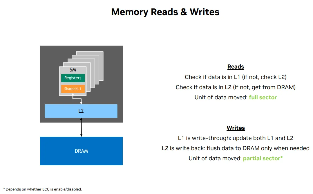
Type
Reads
- Check if data is in L1
- Check if data is in L2
- Get from DRAM
Writes减少不必要的全局内存写入
- L1 is write-through(透写): 当数据被写入 L1 Cache 时,它同时会被写入 L2 Cache或全局内存。这种方式确保数据的一致性,但可能会增加写入延迟,因为每次写入都需要额外的存储操作。
- L2 is write back(回写): flush data to DRAM only when needed. 数据首先写入 L2 Cache,而不会立即写入全局内存。只有当 L2 Cache 需要腾出空间时,数据才会被刷新到全局内存。这种方式减少了写入次数,提高了性能,但可能会导致数据一致性问题,需要额外的同步机制来确保正确性。
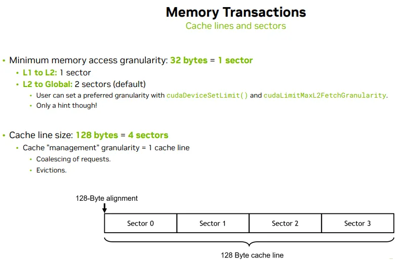
Granularity
| 层级路径 | 粒度 | 传输单位(传输粒度) | 管理单位(缓存粒度) | 说明 |
|---|---|---|---|---|
| Thread → L1 Cache | 访问粒度 | 按需(如 4B、8B) | 无需加载 cache line | 每个线程访问大小决定传输粒度,如果命中直接返回 |
| L1 Cache → L2 Cache | Sector 粒度 | 通常 1 个 Sector(32B) | 128B cache line(4 × 32B) | 缓存行被 sector 分割;按 sector 加载可减少 over-fetch |
| L2 Cache → Global Mem | Sector 粒度 | 默认 2 个 Sector(64B) | 128B cache line | 可通过 cudaDeviceSetLimit(cudaLimitMaxL2FetchGranularity) 设置为 1、2、4 Sector |
| L1 / L2 内部缓存逻辑 | 缓存行粒度 | 传输视场景而定 | 固定为 128B cache line | 即使只访问 4B,也会加载整条 cache line;用于替换和驱逐 |
Reduce frequency
S - Coalesced global memory access
无论是合并(coalesced)还是非合并(uncoalesced)的内存访问,缓存系统的操作仍然是以 cache line(128 字节)为单位进行的
合并内存访问(Coalesced Access)
- 多个线程访问的是 同一个 cache line 内的连续地址。
- 这些访问可以被合并成 一次内存事务,只需加载一个 cache line。
- 高效,带宽利用率高,缓存命中率也更好。
非合并内存访问(Uncoalesced Access)
- 线程访问的是 分散的地址,可能跨越多个 cache lines。
- 当线程访问的地址 不在同一个 cache line 内,每个线程可能会触发一个 独立的内存事务。
- 每个事务会加载一个完整的 128 字节的 cache line,即使线程只需要其中的 4 字节或 8 字节
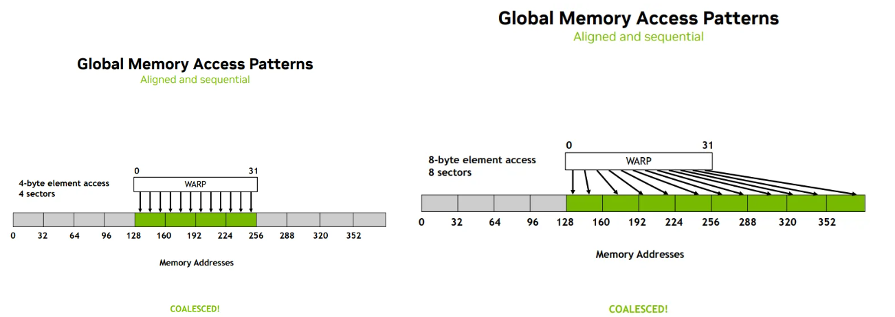
Aligned & Sequential -> Coalesced
Aligned - thread index 0 is at certain memory sector 0
Sequential - thread index and memory address are sequential
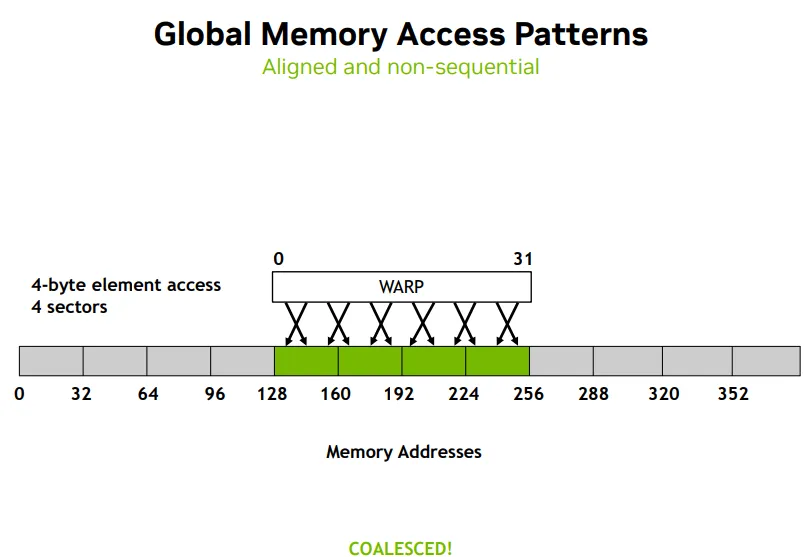
- 32 threads scheduled in a warp
- 4-byte element access: 每个线程访问的是一个 4 字节大小的数据元素,例如 int 或 float 类型。
- 整个 warp 总共访问:32 threads×4 bytes=128 bytes
- 正好等于 一个 cache line 的大小(128 字节),也就是 4 个 sector
- 8 bytes element access -> 8 sectors
Aligned & Non-sequential -> Coalesced
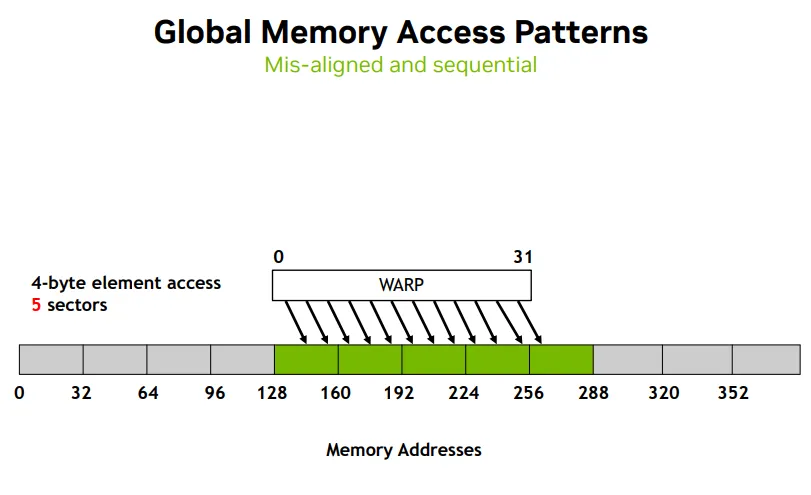
Mis-aligned & Sequential
- need 5 sectors, head and tail sectors not fully-consumed
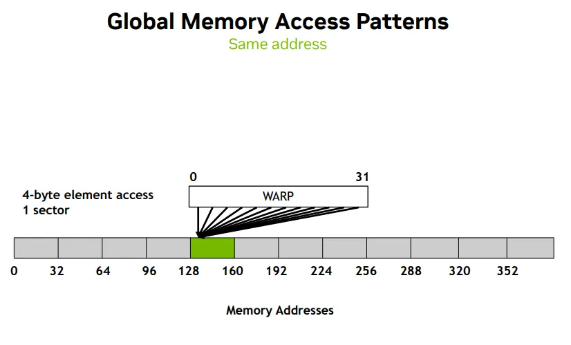
缩小sector数量Same address
- all 32 threads access 1 sector
- 虽然地址 128 到 132 只占用了 4 个字节,但由于内存访问是以 sector(32 字节)为单位 进行的, 所以整个 sector(128 到 160)会被加载
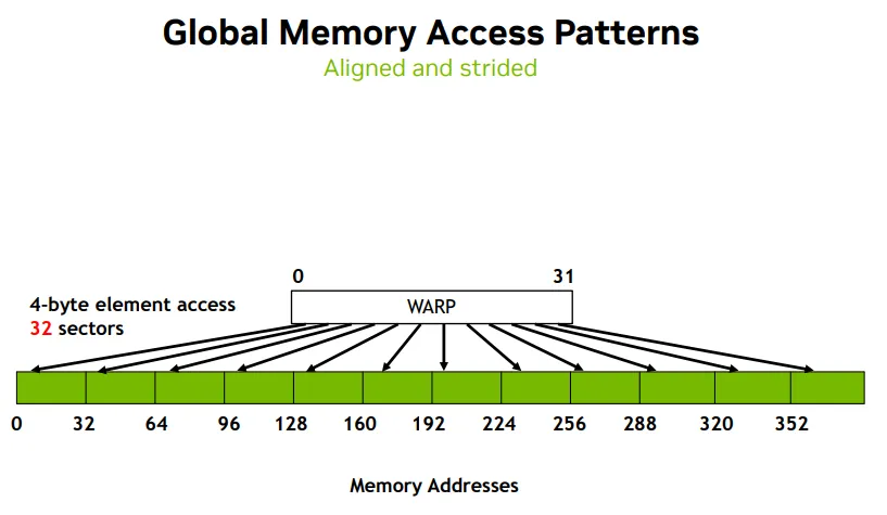
增大sector数量Aligned and strided
- 32 threads access 32 sectors, but 4 byte element access
S - Data Structure/Layout数据布局, Structure-of-Arrays to support coalesced access
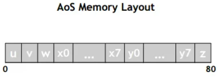
Array-of-Structures(结构体数组)
struct Coefficients {
    float u, v, w;
    float x[8], y[8], z;
};
 结构体定义
结构体定义
- 每个 Coefficients 实例包含多个标量和数组字段
- 所有字段是 混合存储 在一起的
__global__ void kernel(Coefficients *data) {
    int i = cg::this_grid.thread_rank();
    data[i].u = data[i].u + 10.f;
    data[i].y[0] = data[i].y[0] + 10.f;
}
- 每个线程访问 data[i],即结构体数组中的第 i 个元素
- 每个线程访问两个字段:
- u:结构体前部的标量
- y[0]:结构体中部的数组元素
- 性能隐患:AoS 布局的问题
- 每个线程访问的数据(如 data[i].u)在内存中是不连续的
- 这会导致 非合并(uncoalesced)内存访问
- 特别是访问 y[0] 时,线程之间的访问间隔更大,跨越多个 cache line,进一步降低带宽利用率
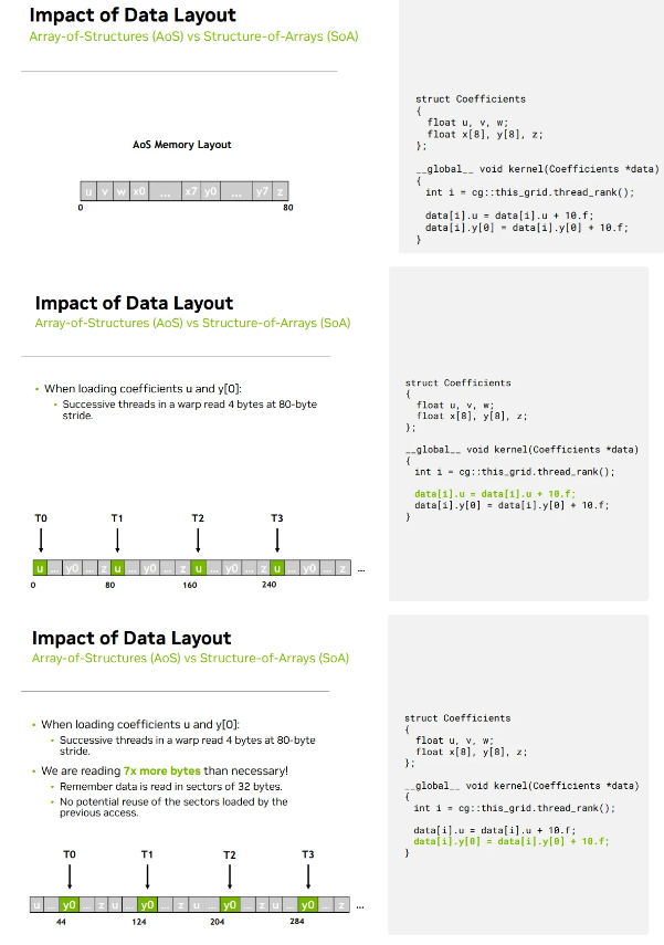
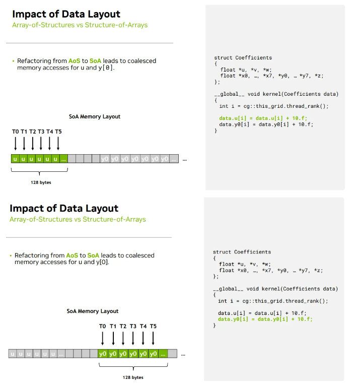
Structure-of-Arrays(数组结构体)
struct Coefficients_SoA {
    float *u, *v, *w;
    float *x[8], *y[8], *z;
};
- 每个字段是一个独立的数组
- 所有线程访问 u[i] 或 y[0][i] 时,地址是连续的
- 可以实现 合并访问(coalesced access),大幅提升性能
Increase parallelism
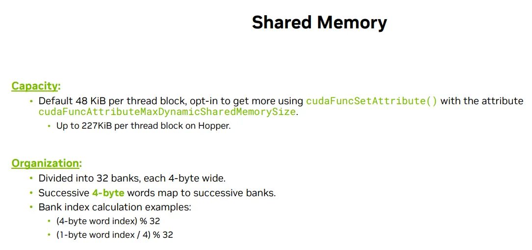
S - Shared memory bank
T - memory bank内存银行
银行强调“并行访问能力”
- 在现实中,一个银行(Bank)可以独立处理客户的请求(如存取款)
- 多个银行可以同时服务多个客户,提高效率
- 每个 memory bank 是一个独立的访问通道
shared memory bank 的设计初衷就是为了提升并行访问能力。它将共享内存划分为多个独立的 bank(通常是 32 个),每个 bank 可以在一个时钟周期内处理一个访问请求。只要多个线程访问的是不同的 bank,就可以实现真正的并行访问;这正是 CUDA 中 warp 内线程高效协同的关键。
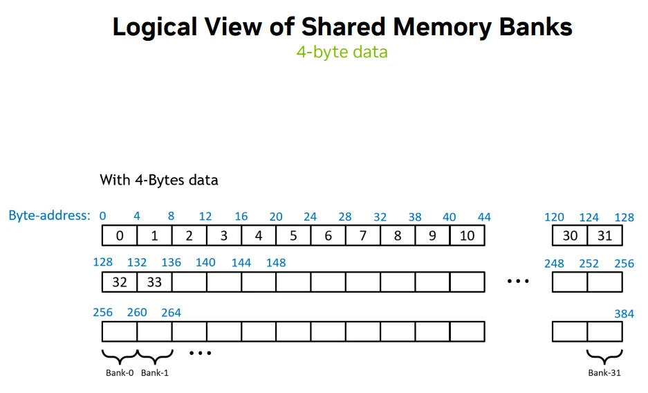
- 4-bytes data -> each bank 4-byte wide
- 128 cache lines -> 128/4=32 bank every line
- 每个bank有多个纵向数据 -> (byte_address / 4) % 32 决定 bank 编号
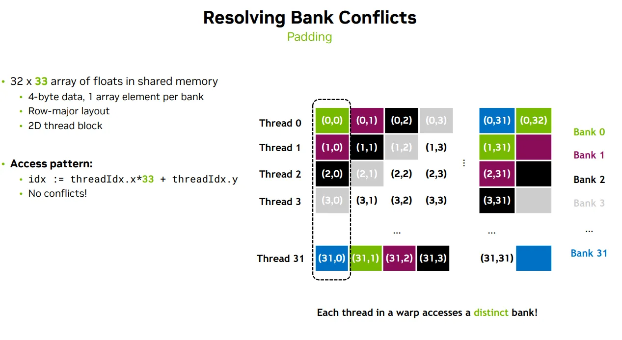
S - Padding & Swizzling to avoid Memory bank conflict
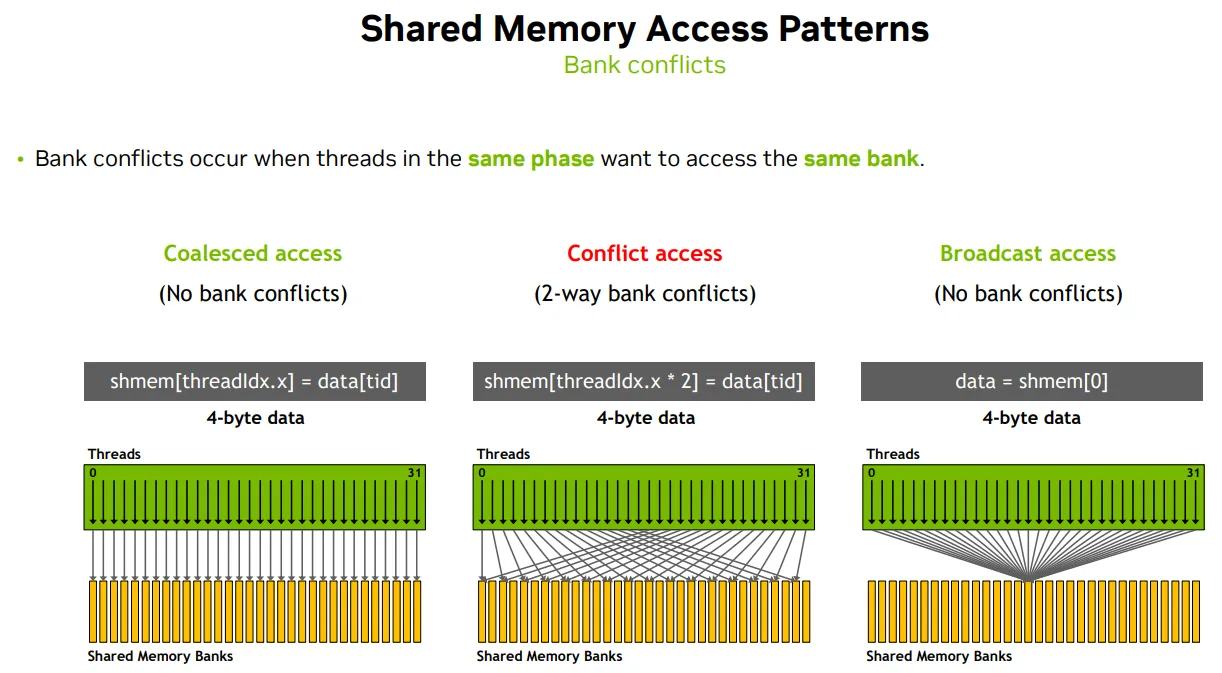
- 如果多个线程访问不同的 bank,就可以并行访问
- 如果多个线程访问同一个 bank,就会发生冲突(bank conflict),访问被串行化
| 访问模式 | 线程地址分布示例 | 映射到 bank 行为 | 是否发生 bank 冲突 | 特殊机制说明 |
|---|---|---|---|---|
shmem[threadIdx.x] = data[tid]; |
线程 0 → bank 0 线程 1 → bank 1 |
每个线程访问不同 bank | ❌ 无冲突 | 并行执行 |
shmem[threadIdx.x * 2] = data[tid]; |
线程 0 → bank 0 线程 1 → bank 2 线程 2 → bank 4 |
地址间隔为 2,但 (addr/4)%32 映射可能重叠 |
⚠️ 2路冲突 | 部分串行化 |
data = shmem[0]; |
所有线程访问 shmem[0] |
同一个地址,映射到同一个 bank | ❌ 无冲突 | ✅ CUDA 广播机制 |
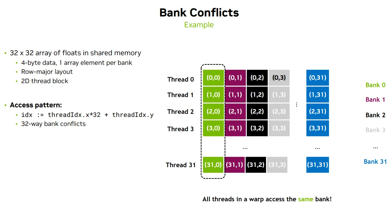
idx = threadIdx.x*32 + threadIdx.y; shmem[idx] |
访问的是二维 shmem 的同一列(如 shmem[0][0~31]) |
⚠️ 32路冲突 |
T - Padding & Swizzling
padding - 在每行末尾填充一个额外元素,打破 bank 对齐
__shared__ float tile[32][33]; // 行数 32,列数 33(第 33 列是 padding)

int idx = threadIdx.x * 33 + threadIdx.y; // 其中每行长度是 33 ➜ 所以需要乘以 33 来正确跳过 padding
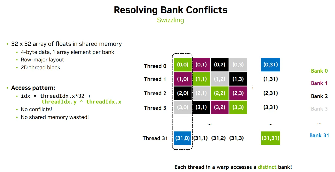
Swizzling - 一种数据重排(data rearrangement)技术
- idx=threadIdx.x*32+(threadIdx.y ^ threadIdx.x);
- 使用了 按位异或(XOR)操作:threadIdx.y ^ threadIdx.x
- 这个操作会打乱原本的列索引,使得每个线程访问的地址映射到 不同的 bank
- 结果是:每个线程访问不同的 bank → 无冲突!
Increase data density
S - Vectorized(Multi-word) access
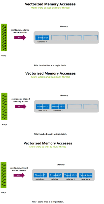
Requirement
Lower precesion
T - Mixed precesion
AMP(Automatic Mixed Precision) 是一种自动使用混合精度(如 float16 和 float32)进行训练的技术
autocast —— 自动切换精度的上下文管理器
- 作用:在 with autocast(): 代码块中,PyTorch 会自动将某些操作(如矩阵乘法、卷积)使用 float16 或 bfloat16 执行,而保留其他操作(如归一化、损失计算)为 float32。
- 好处:无需手动转换张量精度,PyTorch 会根据操作类型和硬件自动选择最优精度。
GradScaler —— 梯度缩放器
- 作用:在使用 float16 时,梯度可能非常小,导致“下溢”(变成 0)。GradScaler 会自动放大 loss,从而放大梯度,避免这种问题。
- 自动管理:它会根据训练情况自动调整缩放因子,确保数值稳定。
A
1.training
model = MyModel().cuda()
optimizer = torch.optim.AdamW(model.parameters(), lr=1e-4)


from torch.cuda.amp import autocast, GradScaler
scaler = GradScaler()


# 训练循环中使用 autocast 和 scaler
for inputs, targets in dataloader:
    inputs, targets = inputs.cuda(), targets.cuda()
    optimizer.zero_grad()

    with autocast():  # 自动使用 float16/bfloat16
        outputs = model(inputs)
        loss = loss_fn(outputs, targets)

    scaler.scale(loss).backward()      # 缩放 loss 以防梯度下溢
    scaler.step(optimizer)             # 更新权重
    scaler.update()                    # 更新缩放因子
2.inference
# 将模型和输入转换为低精度
model.eval()
model.half()  # 或 model.to(torch.bfloat16)
inputs = inputs.half().cuda()

# 使用 autocast 进行推理
with torch.no_grad():
    with autocast():
        outputs = model(inputs)
R
- 著降低内存使用:从 FP32 降到 FP16 或 BF16 可将内存占用减半,允许更大模型或更大 - batch size。
- 提高性能: more thread could be created, high occupancy
- 提升分布式训练效率:低精度减少通信带宽需求,提升多机训练效率。
- 提升训练速度:现代 GPU(如 NVIDIA A100、H100)对低精度计算有专门优化,Tensor Core - 支持 FP16/BF16/FP8。
- 降低能耗与成本:训练 GPT-3 级别模型的成本高达数百万美元,更快速的训练,耗电更少,低精度可显著降低训练成本。