1.2 [PyTorch] MNIST

Problem statement

FashionMNIST Problem Statement

Classify grayscale images of fashion items (e.g., shirts, shoes, bags) into one of 10 categories.
Like MNIST, each image is 28×28 pixels, but the content is clothing-related instead of digits.

MNIST Problem Statement

Classify grayscale images of handwritten digits (0–9) into their correct numeric labels.
Each image is 28×28 pixels, and the task is a 10-class classification problem.

The mainstream PyTorch will solve FashionMNIST probelm. The minor stream of TensorFlow will demostarte how to solve MNIST problem.

Step 1. Data preparation

S - Collecting raw data

FashionMNIST Dataset

Content: 70,000 grayscale images of fashion items (60,000 training + 10,000 test)
Image size: 28×28 pixels
Format: Same binary IDX format as MNIST
- train-images-idx3-ubyte.gz: training images
- train-labels-idx1-ubyte.gz: training labels
- t10k-images-idx3-ubyte.gz: test images
- t10k-labels-idx1-ubyte.gz: test labels
Official link: https://github.com/zalandoresearch/fashion-mnis

MNIST Dataset

Content: 70,000 grayscale images of handwritten digits (60,000 training + 10,000 test) Image size: 28×28 pixels
Format: Binary IDX format (compressed .gz files)
- train-images-idx3-ubyte.gz: training images
- train-labels-idx1-ubyte.gz: training labels
- t10k-images-idx3-ubyte.gz: test images
- t10k-labels-idx1-ubyte.gz: test labels
Official link: http://yann.lecun.com/exdb/mnist/

FashionMNIST is in format of PIL in pytorch namespace MNIST is in format of tensor digits in tensorflow namespace

S - [Tensor lib] How to encode inputs, outputs and paramters of a model

We have raw datasets at hands
How to encode them into the pytorch
This is where is the first core feature of pytorch, tensor lib, comes into play

T - Tensor
torch.Tensor/torch.tensor()

similar to numpy’s ndarrays, support matrix arithmetics
optmized for running on GPUs and automatic differentiation

A Initialize tensor

# 1. from python list
import torch
x_data = torch.tensor([[1,2], [3,4]])


# 2. from numpy array
torch.from_numpy(np.array([[1,2], [3,4]]))


# 3. create random or constant values
shape = (2,3,)
torch.rand(shape)
torch.zeros(shape)
torch.ones(shape)
# Random Tensor:
#  tensor([[0.8918, 0.9173, 0.4270],
#         [0.3927, 0.7944, 0.0999]])
# Zeros Tensor:
#  tensor([[0., 0., 0.],
#         [0., 0., 0.]])
# Ones Tensor:
#  tensor([[1., 1., 1.],
#         [1., 1., 1.]])


# 4. from another tensor
## retain properties (shape and datatype) by default
torch.ones_like(x_data)
#  tensor([[1, 1],
#         [1, 1]])

## override datatype
torch.rand_like(x_data, dtype=torch.float)
#  tensor([[0.7985, 0.1295],
#         [0.4909, 0.2647]])

Data type

#1. tensor's .dtype, to get
## int is python default int64
tensor_int = torch.tensor([1,2])
tensor_int.dtype
# torch.int64

## float is python default float32
torch.tensor([1.0,2.0]).dtype
# torch.float32

#1. tensor's .to(), to convert
## convert int64 to float32
tensor_float = tensor_int.to(torch.float64)
# tensor_int is still torch.int64
# tensor_float is torch.float64, tensor([1., 2.], dtype=torch.float64)

Shape

tensor2d = torch.tensor([[1, 2, 3], 
            [4, 5, 6]])

#1. tensor's .shape, to get
tensor2d.shape
torch.rand(2,3).shape
# Shape of tensor: torch.Size([3, 4])

# pytroch has many syntax to run same function
# initial syntax for Lua version Torch
# new syntax for numpy like

#1.1 tensor's .reshape, to reshape, will auto copy data if not continous
# reshape to 3 * 2
tensor2d.reshape(3,2)
# tensor([[1, 2],
#         [3, 4],
#         [5, 6]])

#1.2 tensor's .view, is more used one, need the raw data is continous in memory
tensor2d.view(3, 2)
# tensor([[1, 2],
#         [3, 4],
#         [5, 6]])

Arithmetics

tensor2d = torch.tensor([[1, 2, 3], 
            [4, 5, 6]])

########### Addition ###########
#1.1 tensor's .sum(), add all values of a tensor into one value
agg = tensor2d.sum() 
# tensor(21)

## .item(), convert single-element tensor to python numerical value
agg_item = agg.item()
print(agg_item, type(agg_item))
# 21 <class 'int'>


#1.2 tensor's .add(), add each value by a same value
tensor2d.add(5)
# tensor2d itself not changed

## tensor's _ suffix, is in-place operations that store result into rhe operand
tensor2d.add_(5)
# tensor2d itself is changed



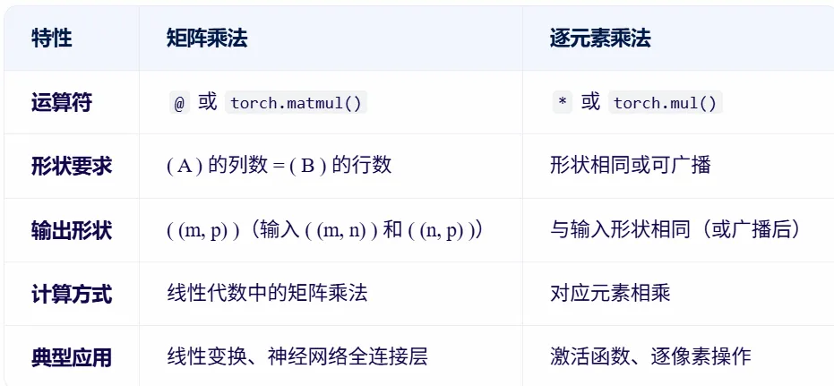
########### When dot product, Matrix Multiplication ###########
#2 tensor's .T, to transpose, interchange row and column
tensor2d.T
# tensor([[1, 4],
#         [2, 5],
#         [3, 6]])

#3.1 tensor's .matmul, matrix multiplication
tensor2d.matmul(tensor2d.T)
# tensor([[14, 32],
#         [32, 77]])

#3.2 @ operator for tensors, more used one
tensor2d @ tensor2d.T
# tensor([[14, 32],
#         [32, 77]])

########### Element-wise Multiplication ###########
# matrix multiplication
A = torch.rand(2, 3)  #  (2, 3)
B = torch.rand(3, 4)  #  (3, 4)
C = A @ B             #  (2, 4)
 
# element-wise multiplication
A = torch.rand(2, 3)  #  (2, 3)
B = torch.rand(2, 3)  #  (2, 3)
D = A * B             #  (2, 3)

alt text

Device

tensor2d = torch.tensor([[1, 2, 3], 
            [4, 5, 6]])

#1. tensor's .device, to get
tensor2d.device
# device(type='cpu')

# by default, tensors are on CPU
#1. tensor's .to(), to explictly move to GPU, copying is expensive in time and memory
device = "cuda" if torch.cuda.is_available() else "cpu"
tensor2d.to(device)

S - Encapsulate tensors and decople for better consumption

We have lots of tensors at hands
Code for processing data samples cane get messy and hard to maintain
How to organize/encapsulate them for better consumption
Decople dataset code from model training code for better readability and modularity

TA - Dataset and Dataloader

We have four torch.Tensor for traning and testing including samples and labels

X_train = torch.tensor([
    [-1.2, 3.1],
    [-0.9, 2.9],
    [-0.5, 2.6],
    [2.3, -1.1],
    [2.7, -1.5]
])

y_train = torch.tensor([0, 0, 0, 1, 1])

X_test = torch.tensor([
    [-0.8, 2.8],
    [2.6, -1.6],
])

y_test = torch.tensor([0, 1])

torch.utils.data.dataset.Dataset/torch.utils.data.Dataset stores the samples and their corresponding labels into one object

Inheritate PyTorch’s Dataset to self define
_ _ init _ _() - initialize properties used by following methods, tensor object
_ _ getitem _ _() - return single sample and label by index
_ _ len _ _() - return samples length

from torch.utils.data import Dataset

class ToyDataset(Dataset):
    def __init__(self, X, y):
        self.features = X
        self.labels = y

    def __getitem__(self, index):
        return self.features[index], self.labels[index]

    def __len__(self):
        return self.labels.shape[0]

train_ds = ToyDataset(X_train, y_train)
test_ds = ToyDataset(X_test, y_test)
# <__main__.ToyDataset object at 0x7f9a7cb46620>


train_ds[0]
# (tensor([-1.2000,  3.1000]), tensor(0))
x, y = test_ds[0][0], test_data[0][1]

torch.utils.data.dataloader.DataLoader/torch.utils.data.DataLoadera() wraps an iterable around the Dateset to enable easy access to the samples.
- batch_size=2
  - improve efficiency
- drop_last=True
  - the last batch may smaller than others, could impact convergence
  - drop the last batch
- shuffle=True
  - Each epoch has same sequence of data, could impact training
  - Shuffle data sequence among epoches
  - use torch.manual_seed(123) to set seed, to get same order of shuffling
- num_workers=4
  - start numtiple worker processes to load data paralelly, to feed GPU

from torch.utils.data import DataLoader

torch.manual_seed(123)

train_loader = DataLoader(
    dataset=train_ds,
    batch_size=2,
    shuffle=True,
    num_workers=0
)

test_loader = DataLoader(
    dataset=test_ds,
    batch_size=2,
    shuffle=False,
    num_workers=0
)
# <torch.utils.data.dataloader.DataLoader object at 0x7f9a7cf0d930>

############ dataloader is an iterable ############
#1. get one batch of data (samples and labels)
i = iter(train_loader) # creates an iterator
data = next(i) # retrieves the first batch from that iterator
# [tensor([[ 2.3000, -1.1000],
#         [-0.9000,  2.9000]]), tensor([1, 0])]
# [tensor(of size 2), tensor(of size 2)]


#2. get each batch of data (samples and labels)
for X, y in test_loader:
    print(X.shape)
    print(y.shape)
    break
# torch.Size([2, 2])
# torch.Size([2])


#3. get one batch of data (samples and labels), with batch index
e = enumerate(test_loader) # enumerator is an interator with index
batch, (X, y) = next(e) 
# (0, [tensor([[-0.8000,  2.8000],
#         [ 2.6000, -1.6000]]), tensor([0, 1])])
# (0, [tensor(of size 2), tensor(of size 2)])


# 4. get each batch of data (samples and labels), with index
for batch_id, (X, y) in enumerate(test_loader):
    print(batch_id)
    print(X.shape)
    print(y.shape)
    break
# 0
# torch.Size([2, 2])
# torch.Size([2])

############ dataloader progress ############
# Batch is based on loader
test_loader
# <torch.utils.data.dataloader.DataLoader object at 0x7f9a7cf0d930>

# 1. total batch num
num_batches = len(test_loader)

# 2. every 100 batch
for batch, (X, y) in enumerate(test_loader): 
    if batch % 100 == 0:
        print(batch)
        # 0,1,2,3,...,60000/64


# data is based on loader.dataset
test_loader.dataset
# <__main__.ToyDataset object at 0x7f9b4e0dcdc0>

# 3. total sample num
len(test_loader.dataset)
# 60000

# 4. current sample num
for batch, (X, y) in enumerate(test_loader): 
    if batch % 100 == 0:
        print((batch + 1) * len(X))

S - Data preprocessing (enhancement, normalization)

Data does not always come in its final processed form that is required for training machine learning algorithms
Need to perform some manipulation of the data and make it suitable for training

T - transform

Load the pre-defined FashionMNIST datasets from torchvision.datasets.FashionMNIST()

encapsulate raw data by datasets
root - is the path where the train/test data is stored
train - specifies training or test dataset
download=True - downloads the data from the internet if it’s not available at root

Preprocessing the datasets

transforms - We use transforms to perform some manipulation of the data and make it suitable for training.

FashionMNIST	Features	Labels
Original	in PIL Image format	integers
Parameter. Both accept callables containing the transformation logic	transform to modify the features	target_transform to modify the labels
Callables	ToTensor() converts a PIL image into a FloatTensor and scales the image’s pixel intensity values in the range [0., 1.] `transform=ToTensor(),`	Lambda transforms apply any user-defined lambda function. Here, we define a function to turn the integer into a one-hot encoded tensor. It first creates a zero tensor of size 10 (the number of labels in our dataset) and calls scatter_ which assigns a value=1 on the index as given by the label y. `py target_transform = Lambda(lambda y: torch.zeros(10, dtype=torch.float).scatter_(dim=0, index=torch.tensor(y), value=1))`
Trainig req	as normalized tensors	as one-hot encoded tensors.

A2 - PT on MNIST

from torchvision import datasets
from torchvision.transforms import ToTensor

# Download training data from open datasets.
training_data = datasets.FashionMNIST(
    root="data",
    train=True,
    download=True,
    transform=ToTensor(),
)

# Download test data from open datasets.
test_data = datasets.FashionMNIST(
    root="data",
    train=False,
    download=True,
    transform=ToTensor(),
)

from torch.utils.data import DataLoader

batch_size = 3

train_dataloader = DataLoader(training_data, batch_size=batch_size)
test_dataloader = DataLoader(test_data, batch_size=batch_size)

A2 - TF on MNIST

Load the MNIST from tf.keras.datasets.mnist.load_data() Originally

pixel values of the images range from 0 through 255
they are all numpy.ndarray

Normalization

Scale these values to a range of 0 to 1 by dividing the values by 255.0.
Above also converts the sample data from integers to floating-point numbers

import tensorflow as tf

mnist = tf.keras.datasets.mnist

(x_train, y_train), (x_test, y_test) = mnist.load_data()
x_train, x_test = x_train / 255.0, x_test / 255.0

Summary

from torchvision import datasets
from torchvision.transforms import ToTensor
from torch.utils.data import DataLoader

batch_size = 3

# Download training data from open datasets.
training_data = datasets.FashionMNIST(
    root="data",
    train=True,
    download=True,
    transform=ToTensor(),
)

# Download test data from open datasets.
test_data = datasets.FashionMNIST(
    root="data",
    train=False,
    download=True,
    transform=ToTensor(),
)

train_dataloader = DataLoader(training_data, batch_size=batch_size)
test_dataloader = DataLoader(test_data, batch_size=batch_size)

import tensorflow as tf

mnist = tf.keras.datasets.mnist

(x_train, y_train), (x_test, y_test) = mnist.load_data()
x_train, x_test = x_train / 255.0, x_test / 255.0

Step2. Model definition

S - [DL lib] Define the model/neural network

T - DL lib torch.nn namespace provides all the building blocks you need to build your own neural network

inherits from nn.Module
_ _ init _ _() function - define the layers of the network
forward function - specify how data will pass through the network. This forms the computing graph
move the model also to the accelerator.

Input - a sample minibatch of 3 images of size 28x28

input_image = torch.rand(3,28,28)
print(input_image.size())
# torch.Size([3, 28, 28])

initialize the nn.Flatten layer to convert each 2D 28x28 image into a contiguous array of 784 pixel values

flatten = nn.Flatten()
flat_image = flatten(input_image)
print(flat_image.size())
# torch.Size([3, 784])

nn.Linear layer is a module that applies a linear transformation on the input using its stored weights and biases.

layer1 = nn.Linear(in_features=28*28, out_features=20)
hidden1 = layer1(flat_image)
print(hidden1.size())
# torch.Size([3, 20])

nn.ReLU non-linear activations are applied after linear transformations to introduce nonlinearity, helping neural networks learn a wide variety of phenomena.

print(f"Before ReLU: {hidden1}\n\n")
hidden1 = nn.ReLU()(hidden1)
print(f"After ReLU: {hidden1}")

nn.Sequential is an ordered container of modules. The data is passed through all the modules in the same order as defined.

seq_modules = nn.Sequential(
    flatten,
    layer1,
    nn.ReLU(),
    nn.Linear(20, 10)
)

from torch import nn

# Define model
class NeuralNetwork(nn.Module):
    def __init__(self):
        super().__init__()
        self.flatten = nn.Flatten()
        self.linear_relu_stack = nn.Sequential(
            nn.Linear(28*28, 512),
            nn.ReLU(),
            nn.Linear(512, 512),
            nn.ReLU(),
            nn.Linear(512, 10)
        )

    def forward(self, x):
        x = self.flatten(x)
        logits = self.linear_relu_stack(x)
        return logits

import torch
device = torch.device("cuda" if torch.cuda.is_available() else "cpu")
model = NeuralNetwork().to(device)
print(model)
# NeuralNetwork(
#   (flatten): Flatten(start_dim=1, end_dim=-1)
#   (linear_relu_stack): Sequential(
#     (0): Linear(in_features=784, out_features=512, bias=True)
#     (1): ReLU()
#     (2): Linear(in_features=512, out_features=512, bias=True)
#     (3): ReLU()
#     (4): Linear(in_features=512, out_features=10, bias=True)
#   )
# )

# Every param with requires_grad=True will be trained and updated ruding training.
# Accee weight of one layer
model.layers[0].weight
# Accee bias of one layer
model.layers[0].bias
# Check all trainable params of one model
sum(p.numel() for p in model.parameters() if p.requires_grad)

PT: nn.Linear(in_features, out_features)

in_features: input dimension
out_features: output dimension = number of neurons in the layer

TF: tf.keras.layers.Dense(units)

units: Number of neurons in the layer = output dimension
Input dimension is inferred from the previous layer or specified using input_shape.

model = tf.keras.models.Sequential([
  tf.keras.layers.Flatten(input_shape=(28, 28)),
  tf.keras.layers.Dense(128, activation='relu'),
  tf.keras.layers.Dense(10)
])

Step3. Training loop

S - Move data and model to GPU

model = model.to(device)

for batch, (X, y) in enumerate(dataloader):
    X, y = X.to(device), y.to(device)

S - Training

T 1. Put model in training mode

model.train()

📌 Evaluation turns off dropout model.eval()

📌 Inference turns off dropout model.eval()

2. Forward pass/predict alt text Dynamic computation graph

Dynamic
- Computation graph is constructed on-the-fly when you really forward pass.
- Every foward pass will build a new computation graph to accomodate current input data
Computation graph
- Is a directed graph
- List all the computing sequnce, which will be used later to calculate gradient when backpropagation.
How
- As long as one of the end node is set with required_grad=True, PyTorch will build a computing graph by default accroding to foward().

pred = model(X)
# tensor([[-1.0240e-01,  6.9089e-02,  ...

How to use the pred result

pred = model(x)
pred
# tensor([[-2.6683, -3.2515, -1.3364, -2.3363, -1.3656,  3.0426, -1.2521,  3.0325,
#           2.0545,  3.5086]], grad_fn=<AddmmBackward0>)

pred[0]
# tensor([-2.6683, -3.2515, -1.3364, -2.3363, -1.3656,  3.0426, -1.2521,  3.0325,
#          2.0545,  3.5086], grad_fn=<SelectBackward0>)

pred[0].argmax(0)
# tensor(9)

# if pred is a matrix
# (pred.argmax(1) == y).type(torch.float).sum().item()

📌 Evaluation No backpropagation, no training, no need to build computation graph to save memory with torch.no_grad(): out = model(X)

📌 Inference No backpropagation, no training, no need to build computation graph to save memory with torch.no_grad(): out = model(X)

3. Calculate loss/prediction error with Loss function (CrossEntropyLoss, MSELoss) Return logits in last layer in pytorch

Pytorch’s loss function (CrossEntropyLoss) will apply softmax for logits internally, and use more stable way like log-softmax + NLLLoss to avoid overflow and underflow

loss_fn = nn.CrossEntropyLoss()
loss = loss_fn(pred, y)
# tensor(2.3065, grad_fn=<NllLossBackward0>)

📌 Evaluation Need this step to show loss only.

📌 Inference No need this step. But need to softmax the output logits=[2.0,1.0,0.1] probs=softmax(logits)

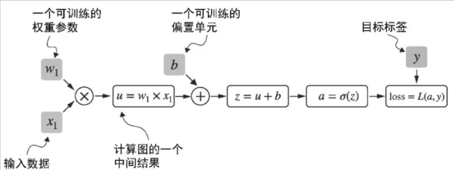
4. Backpropogation to compute gradient Calculate loss’s garident to w1 by grad()

import torch.nn.functional as F
from torch.autograd import grad

y = torch.tensor([1.0])
x1 = torch.tensor([1.1])
w1 = torch.tensor([2.2], requires_grad=True)
b = torch.tensor([0.0], requires_grad=True)

z = x1 * w1 + b 
a = torch.sigmoid(z)

loss = F.binary_cross_entropy(a, y)

grad_L_w1 = grad(loss, w1, retain_graph=True)
grad_L_b = grad(loss, b, retain_graph=True)

print(grad_L_w1)
print(grad_L_b)

# (tensor([-0.0898]),)
# (tensor([-0.0817]),)

PyTorch provides Autograd to automate this process: loss.backward()

Compute the gradients of all leaf nodes in the computation graph.
These gradients are stored in the .grad attribute of the tensors

loss.backward()

print(w1.grad)
print(b.grad)
# tensor([-0.0898])
# tensor([-0.0817])

📌 Evaluation No need this step.

📌 Inference No need this step.

5. Update parameters with Optimizer (SGD, Adam, AdamW)

optimizer = torch.optim.SGD(model.parameters(), lr=1e-3)
# params：params to be optimized, normally model.parameters()
# lr：learning rate

# Gradients accumulate by default in PyTorch (i.e., they are not overwritten), so you need to zero them out before the next backward pass.
optimizer.zero_grad()

# Computes the gradients of the loss with respect to all model parameters (i.e., performs backpropagation).
# loss.backward()

# Applies the optimization algorithm (e.g., SGD, Adam) to adjust the weights to minimize the loss.
optimizer.step()

📌 Evaluation No need this step.

📌 Inference No need this step.

S - Epochs loop

epochs = 5
for t in range(epochs):
    print(f"Epoch {t} ------------------------------")
    train()

Summary

def train(dataloader, model, loss_fn, optimizer):
    model.train()
    for batch, (X, y) in enumerate(dataloader):
        X, y = X.to(device), y.to(device)

        # Compute prediction error
        pred = model(X)
        loss = loss_fn(pred, y)

        # Backpropagation
        optimizer.zero_grad()
        loss.backward()
        optimizer.step()  

loss_fn = nn.CrossEntropyLoss()
optimizer = torch.optim.SGD(model.parameters(), lr=1e-3)

epochs = 5
for t in range(epochs):
    print(f"Epoch {t} ------------------------------")
    train(train_dataloader, model, loss_fn, optimizer)

TF on MNIST Why from_logits=True?

If your model’s final layer does not include a Softmax activation (i.e., it outputs raw scores or “logits”), you must set from_logits=True.
This tells TensorFlow to apply softmax internally before computing the cross-entropy loss.

loss_fn = tf.keras.losses.SparseCategoricalCrossentropy(from_logits=True)
optimizer='adam'

model.compile(optimizer='adam',
              loss=loss_fn,
              metrics=['accuracy'])

model.fit(x_train, y_train, epochs=5)

Step 5. Model usage/inference

classes = [
    "T-shirt/top",
    "Trouser",
    "Pullover",
    "Dress",
    "Coat",
    "Sandal",
    "Shirt",
    "Sneaker",
    "Bag",
    "Ankle boot",
]

model.eval()
x, y = test_data[0][0], test_data[0][1]
with torch.no_grad():
    x = x.to(device)
    pred = model(x)
    predicted, actual = classes[pred[0].argmax(0)], classes[y]
    print(f'Predicted: "{predicted}", Actual: "{actual}"')

Step 5.Model evaluation

S - Show progress with loss and accuracy

T Train Every 100 batch and overall data process, show the loss alt text

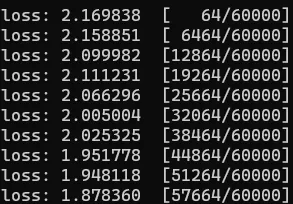
>7f denotes
  > right aligned
  7 overall width is 7 chars
  f show float

size = len(dataloader.dataset)
for batch, (X, y) in enumerate(dataloader):
    if batch % 100 == 0:
        loss, current = loss.item(), (batch + 1) * len(X)
        print(f"loss: {loss:>7f}  [{current:>5d}/{size:>5d}]")

Test Each epoch, show average loss by batch

test_loss = 0
for every batch:
    test_loss += loss_fn(pred,y).item()
num_batches = len(dataloader)
test_loss /= num_batches

Each epoch, show the accurate sample number

correct = 0
for:
    correct += (pred.argmax(1) == y).type(torch.float).sum().item()
size = len(dataloader.dataset)
correct /= size

pred.argmax(1)：get index of highest value
== y：compare with target
.type(torch.float): convert bool to float
.sum(): sum each sample
.item(): covnert to python datatype

def train(dataloader, model, loss_fn, optimizer):
    size = len(dataloader.dataset)
    model.train()
    for batch, (X, y) in enumerate(dataloader):
        X, y = X.to(device), y.to(device)

        # Compute prediction error
        pred = model(X)
        loss = loss_fn(pred, y)

        # Backpropagation
        optimizer.zero_grad()
        loss.backward()
        optimizer.step()

        if batch % 100 == 0:
            loss, current = loss.item(), (batch + 1) * len(X)
            print(f"loss: {loss:>7f}  [{current:>5d}/{size:>5d}]")

def test(dataloader, model, loss_fn):
    size = len(dataloader.dataset)
    num_batches = len(dataloader)
    test_loss, correct = 0, 0

    model.eval()
    with torch.no_grad():
        for X, y in dataloader:
            X, y = X.to(device), y.to(device)
            pred = model(X)
            test_loss += loss_fn(pred, y).item()
            correct += (pred.argmax(1) == y).type(torch.float).sum().item()
    test_loss /= num_batches
    correct /= size
    print(f"Test Error: \n Accuracy: {(100*correct):>0.1f}%, Avg loss: {test_loss:>8f} \n")

loss_fn = nn.CrossEntropyLoss()
optimizer = torch.optim.SGD(model.parameters(), lr=1e-3)

epochs = 5
for t in range(epochs):
    print(f"Epoch {t}------------------------------")
    train(train_dataloader, model, loss_fn, optimizer)
    test(test_dataloader, model, loss_fn)
print("Done!")

TF on MNIST

model.evaluate(x_test,  y_test, verbose=2)

Step 6. Model checkpoint save and load

T
Model has

structure
internal state dictionary (containing the model parameters)
像 AdamW 这样的自适应优化器可以为每个模型权重存储额外的参数。AdamW 可以使用历史数据动态地调整每个模型参数的学习率。

Save a model

is to serialize the internal state dictionary to a file .pth

Load a model includes

re-creating the model structure
loading the state dictionary into it.

torch.save(model.state_dict(), "model.pth")

model = NeuralNetwork().to(device)
model.load_state_dict(torch.load("model.pth", weights_only=True))

# save
torch.save({
    "model_state_dict": model.state_dict(),
    "optimizer_state_dict": optimizer.state_dict(),
    }, 
    "model_and_optimizer.pth"
)

# load
checkpoint = torch.load("model_and_optimizer.pth", weights_only=True)

model = GPTModel(GPT_CONFIG_124M)
model.load_state_dict(checkpoint["model_state_dict"])

optimizer = torch.optim.AdamW(model.parameters(), lr=0.0005, weight_decay=0.1)
optimizer.load_state_dict(checkpoint["optimizer_state_dict"])

model.train()

Conclusion

from torchvision import datasets
from torchvision.transforms import ToTensor

# Download training data from open datasets.
training_data = datasets.FashionMNIST(
    root="data",
    train=True,
    download=True,
    transform=ToTensor(),
)

# Download test data from open datasets.
test_data = datasets.FashionMNIST(
    root="data",
    train=False,
    download=True,
    transform=ToTensor(),
)


from torch.utils.data import DataLoader

batch_size = 3

# Create data loaders.
train_dataloader = DataLoader(training_data, batch_size=batch_size)
test_dataloader = DataLoader(test_data, batch_size=batch_size)



from torch import nn

# Define model
class NeuralNetwork(nn.Module):
    def __init__(self):
        super().__init__()
        self.flatten = nn.Flatten()
        self.linear_relu_stack = nn.Sequential(
            nn.Linear(28*28, 512),
            nn.ReLU(),
            nn.Linear(512, 512),
            nn.ReLU(),
            nn.Linear(512, 10)
        )

    def forward(self, x):
        x = self.flatten(x)
        logits = self.linear_relu_stack(x)
        return logits

import torch
device = torch.device("cuda" if torch.cuda.is_available() else "cpu")
model = NeuralNetwork().to(device)
print(model)



def train(dataloader, model, loss_fn, optimizer):
    size = len(dataloader.dataset)
    model.train()
    for batch, (X, y) in enumerate(dataloader):
        X, y = X.to(device), y.to(device)

        # Compute prediction error
        pred = model(X)
        loss = loss_fn(pred, y)

        # Backpropagation
        loss.backward()
        optimizer.step()
        optimizer.zero_grad()

        if batch % 100 == 0:
            loss, current = loss.item(), (batch + 1) * len(X)
            print(f"loss: {loss:>7f}  [{current:>5d}/{size:>5d}]")




def test(dataloader, model, loss_fn):
    size = len(dataloader.dataset)
    num_batches = len(dataloader)
    model.eval()
    test_loss, correct = 0, 0
    with torch.no_grad():
        for X, y in dataloader:
            X, y = X.to(device), y.to(device)
            pred = model(X)
            test_loss += loss_fn(pred, y).item()
            correct += (pred.argmax(1) == y).type(torch.float).sum().item()
    test_loss /= num_batches
    correct /= size
    print(f"Test Error: \n Accuracy: {(100*correct):>0.1f}%, Avg loss: {test_loss:>8f} \n")




loss_fn = nn.CrossEntropyLoss()
optimizer = torch.optim.SGD(model.parameters(), lr=1e-3)


epochs = 5
for t in range(epochs):
    print(f"Epoch {t}\n-------------------------------")
    train(train_dataloader, model, loss_fn, optimizer)
    test(test_dataloader, model, loss_fn)
print("Done!")




classes = [
    "T-shirt/top",
    "Trouser",
    "Pullover",
    "Dress",
    "Coat",
    "Sandal",
    "Shirt",
    "Sneaker",
    "Bag",
    "Ankle boot",
]

model.eval()
x, y = test_data[0][0], test_data[0][1]
with torch.no_grad():
    x = x.to(device)
    pred = model(x)
    predicted, actual = classes[pred[0].argmax(0)], classes[y]
    print(f'Predicted: "{predicted}", Actual: "{actual}"')

import tensorflow as tf

mnist = tf.keras.datasets.mnist

(x_train, y_train), (x_test, y_test) = mnist.load_data()
x_train, x_test = x_train / 255.0, x_test / 255.0



model = tf.keras.models.Sequential([
  tf.keras.layers.Flatten(input_shape=(28, 28)),
  tf.keras.layers.Dense(128, activation='relu'),
  tf.keras.layers.Dropout(0.2),
  tf.keras.layers.Dense(10)
])


loss_fn = tf.keras.losses.SparseCategoricalCrossentropy(from_logits=True)
optimizer='adam'

model.compile(optimizer='adam',
              loss=loss_fn,
              metrics=['accuracy'])

model.fit(x_train, y_train, epochs=5)


model.evaluate(x_test,  y_test, verbose=2)

Problem statement#

Step 1. Data preparation#

S - Collecting raw data#

S - [Tensor lib] How to encode inputs, outputs and paramters of a model#

S - Encapsulate tensors and decople for better consumption#

S - Data preprocessing (enhancement, normalization)#

Summary#

Step2. Model definition#

S - [DL lib] Define the model/neural network#

Step3. Training loop#

S - Move data and model to GPU#

S - Training#

S - Epochs loop#

Summary#

Step 5. Model usage/inference#

Step 5.Model evaluation#

S - Show progress with loss and accuracy#

Step 6. Model checkpoint save and load#

Conclusion#

Problem statement

Step 1. Data preparation

S - Collecting raw data

S - [Tensor lib] How to encode inputs, outputs and paramters of a model

S - Encapsulate tensors and decople for better consumption

S - Data preprocessing (enhancement, normalization)

Summary

Step2. Model definition

S - [DL lib] Define the model/neural network

Step3. Training loop

S - Move data and model to GPU

S - Training

S - Epochs loop

Summary

Step 5. Model usage/inference

Step 5.Model evaluation

S - Show progress with loss and accuracy

Step 6. Model checkpoint save and load

Conclusion